Interactive figure
Inventory problems as network diagrams
Requests, supply, lead-time pipelines, allocation, waste, and backlog can be drawn as one graph language. The learning recipe changes the controlled arcs, not the abstraction.
Summary
- One generic recipe — Covariance Matrix Adaptation Evolution Strategies (CMA-ES) optimizing small, interpretable policies — learns competitive inventory-control policies across ten classical problems, with little tuning.
- The learned policies are tiny: tens to a few hundred parameters, orders of magnitude smaller than the deep networks usually reported, and small enough to read.
- The recurring trick is that the action parameterization is part of the policy: the decoder is shaped like the relevant heuristic’s coordinate system, which is what lets such a small policy reach the good operating region.
This post started life as a tutorial on the lost-sales problem alone. Since then the study has broadened: the same loop now runs, essentially unchanged, across ten structurally different inventory problems. I lead with lost sales — still the most developed example — and then widen out.
The setup: a sequential decision under uncertainty
Inventory management is a textbook sequential decision problem. Each period a controller decides how much to order, balancing the cost of holding stock against the cost of shortages. These problems are naturally Markov decision processes (MDPs), but exact dynamic programming is only tractable for small instances — the state space grows with the lead time and the number of stocking locations (the curse of dimensionality). So the field leans on two things:
- Problem-specific heuristics — base-stock, $(s,S)$, $(s,nQ)$, dual-index, capped dual-index. These are strong, but each one takes specialized analysis and simplifying assumptions that limit where it applies.
- Deep reinforcement learning (DRL) — represent the policy as a neural network and tune it from simulated experience (the line opened up for inventory by Boute et al.’s 2022 roadmap and Gijsbrechts et al.’s 2022 cross-problem study). This is generic, but it demands a lot of compute and hyperparameter tuning, and the networks (thousands to millions of parameters) are hard to interpret. I come back to where this literature is heading below.
The question I want to ask here is different from “what is the best method for problem X”. It is: can one lightweight, portable recipe stand in for bespoke heuristics across many different inventory problems, while staying small enough to interpret and cheap enough to retrain?
The recipe is to optimize the parameters of a compact policy with CMA-ES, a gradient-free, population-based optimizer. Three things make it a good fit, and they hold across all ten problems:
- It optimizes the realized objective — the simulated long-run average cost — directly. No value-function bootstrapping, no reward shaping, no credit assignment to individual actions. The same loop applies whether the action is a scalar order, a regular/expedite pair, or a pair of echelon order-up-to levels.
- Its built-in covariance adaptation supplies exploration automatically, so there is no exploration strategy to design.
- Because it never differentiates the policy, it happily handles the non-smooth, discretized, clipped action maps that are awkward for backpropagation but completely natural for inventory controls.
A note on continuity from the original post: the earlier version pitched ES against RL specifically for lost sales. The thesis here is the same in spirit but bigger in scope — it is the portability of one recipe across ten problems that is the point, not a single head-to-head on one problem.
The training loop
CMA-ES is treated as a black-box optimizer. Each generation does three things: it samples a population of policy-parameter vectors from a Gaussian search distribution; it evaluates each one by short rollouts in the simulator (the only step that touches the environment), giving a simulated long-run cost; and it ranks and updates the search distribution from the best members. We use a single fixed configuration throughout (population 64, a short 2000-period training horizon) and do not tune it per problem.
es = CMAES(num_params=num_params, popsize=64)
for generation in range(num_generations):
    candidates = es.ask()                      # sample a population of policies
    costs = [rollout_cost(decode(c)) for c in candidates]  # evaluate each (parallelizable)
    es.tell(costs)                             # update mean, step size, covariance
The evaluation step is embarrassingly parallel — one of ES’s structural advantages over RL — so it scales cleanly across cores or a cluster.
How every result is reported: seed-robust, by honest verdict
Two reporting rules are the methodological backbone of everything below, and they are worth stating up front because they change which claims survive.
- Every learned result is a mean ± standard deviation over five independent optimizer seeds — never a single seed and never best-of-N. CMA-ES is stochastic, so a single run can land lucky; the honest signal is the cross-seed distribution. A learned policy is only credited with a beat when the seed-mean margin clears the cross-seed std (ideally with every seed on the winning side), all under a paired common-random-number (CRN) comparison against the same-protocol gate. This discipline is not cosmetic: it is what turned an earlier single-seed dual-sourcing “beats CDI on two rows” into an honest match, and conversely what let the production network’s mixed variant go from a noisy tie to a robust beat once a new decoder collapsed the seed scatter.
- Each problem is read by one of four honest verdicts, never a single ”% improvement” leaderboard: match a proven optimum or near-optimal proxy (never “beat”), beat a heuristic gate (margin clears the held-out error), report a gap to an upper bound (reported, never “beaten”), or a research result against an environment’s own best heuristic on a faithful-but-not-literature-anchored environment. Where the comparator is published deep RL (A3C, PPO, DRL), it is cross-protocol context only — a different learner under a different protocol — and is never claimed as a head-to-head beat.
The key idea: the action parameterization is the policy
This is the one idea worth taking away, and it runs through every problem.
A learner that can only emit a raw scalar order is implicitly restricted to whatever that scalar can express. A learner whose decoder is shaped like the relevant structured heuristic searches a far more useful action geometry. So I treat each policy as a single map from the problem’s state to a valid action, and everything in between — a divide-by-scale normalization, a small backbone (a linear map, a one-hidden-layer network, or a soft decision tree), and crucially a decoder / action geometry — is owned by the policy and learned by CMA-ES.
Where a structured heuristic exists, the decoder lives in that heuristic’s coordinate system:
- an ordinal “one more unit” quantity for lost sales,
- capped-dual-index coordinates for dual sourcing,
- direct echelon order-up-to levels for multi-echelon.
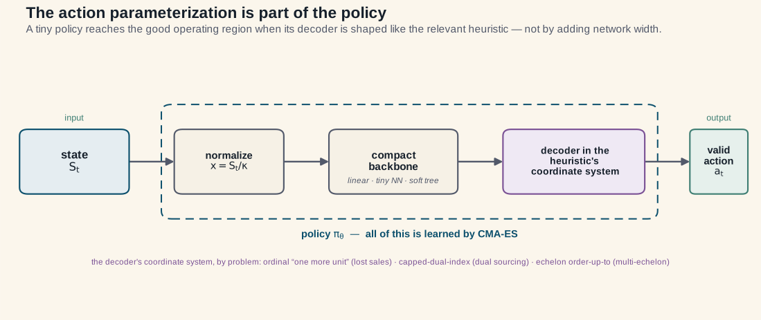
The payoff is that the decoder, not the network width, drives several of the results. The clearest example is multi-echelon (below): with the same tree, optimizer and horizon, changing only the decoder’s reachable action set swings the policy from ~14% better than the best base-stock to more than 200% worse.
Lost sales (the original problem)
The lost-sales problem is one of the fundamental problems in inventory theory. Single item, periodic review, integer demand and orders. Each period: an order placed $L$ periods ago arrives and joins on-hand stock; the controller places a new integer order $q_t$ that will arrive after lead time $L$; demand $D_t$ is realized and served from stock, and any unmet demand is lost rather than backordered. A holding cost $h$ is charged per leftover unit and a penalty $p$ per lost unit:
$$ c_t = h,(I_t - D_t)^{+} + p,(D_t - I_t)^{+}. $$
The state is the on-hand inventory plus the pipeline of outstanding orders, an $L$-dimensional vector — and the state space grows exponentially in the lead time, which is exactly why exact solution is intractable and the problem is famously hard.
The action here is a single integer order, so this is where the decoder family lives. We use three policy-owned decoders: a soft-gated direct quantity (a logistic gate decides whether to order, a softplus head decides how much), a soft-gated ordinal quantity (a sum of soft “one more unit” indicators), and soft decision trees with linear leaves.
We benchmark on a surface, not a single instance: holding cost 1, mean demand 5, lead times $L\in{4,6,8,10}$, lost-sales penalties $p\in{4,19}$, and three mean-preserving demand families (Poisson, Geometric, and a positively-correlated Markov-modulated Poisson). That is 24 vanilla instances. The comparators are the strong classical heuristics: Myopic-1, Myopic-2, and standard vector base-stock.
Result. Across the 24-instance vanilla surface, the learned policies are instance-best in 22 of 24 cases. The soft tree is the most frequent winner. The two cases still won by a classical baseline are the high-penalty, autocorrelated MMPP instances at the longest lead times ($L=8,10$) — a regime-switching, deep-pipeline combination that is the hardest setting for a single stationary compact policy.
Fixed-cost lost sales
Add a fixed setup cost $K$ charged whenever a strictly positive order is placed, and the order/no-order decision becomes an explicit part of the problem — it is no longer optimal to order every period. The comparators become the $(s,S)$, $(s,nQ)$, and modified $(s,S,q)$ policies; the surface grows to 48 instances with $K\in{5,25}$.
Result. Learned policies are instance-best in 47 of 48 instances. And the architecture story sharpens: once a setup charge makes the order/no-order boundary dominant, the gated decoders — which factor the decision into an explicit gate (whether) and a quantity head (how much) — win most instances, inverting the vanilla preference. There is an honest failure mode visible right in the table: at high setup cost a couple of the decoders collapse onto a degenerate “never order” policy; the gated ordinal decoder is the one that consistently escapes it. The decoder, not the optimizer, governs that boundary.
Broadening out: the other eight problems
The same loop, the same optimizer configuration, the same idea — only the decoder and the action geometry change.
Dual sourcing — the heuristic-near-optimal anchor, matched
Two supply modes (a cheap slow regular source and an expensive fast expedited one). On the six small benchmark instances of Gijsbrechts et al. (2022), the strongest structured policy is the capped dual-index (CDI) heuristic, whose published optimality gap is $\le 0.11%$. This is the post’s heuristic-near-optimal anchor: a separate bounded-DP sweep across the reachable regime confirms CDI is within roughly $0.4%$ of the exact optimum everywhere it can be validated (the largest gap demonstrated anywhere is $+0.305%$ single-path / $+0.160%$ out-of-sample, and there is no $\ge 5%$ “hard” regime — an honest negative). So CDI is, for all practical purposes, an optimal proxy, and the right verdict here is match, not beat.
By putting the learned soft tree in capped-dual-index coordinates and warm-starting CMA-ES at the CDI solution, the learned policy matches CDI on all six instances under the seed-robust standard (mean ± std over five optimizer seeds). The seed-mean relative gap to CDI runs from +0.09% ± 0.13% on the two tightest rows to +0.96% ± 0.84% on the loosest — i.e. every row’s seed-mean sits at or just above CDI, well inside CDI’s own optimality band. I report this as a match, not an improvement: an earlier single-seed read showed two rows a hair below CDI (by 0.009% and 0.041%), but over five seeds that was a best-of-the-noise straddle inside the band, not a robust beat — no row robustly beats CDI, and at the hardest reachable cell the learned policy does not even robustly match it (CDI wins, 0/5). As indicative context, the published A3C learner sits at a 0.51–1.85% gap, i.e. outside the band the learned policy lands in — but A3C is a different protocol and is context, not a head-to-head beat. The lever here is the action geometry: a raw direct-order decoder cannot express CDI and does not reach this level.
Divergent multi-echelon with special delivery — 14.7% / 12.0% over the best base-stock
One warehouse, $R$ retailers, with a special-delivery option. The action is a warehouse order plus a shared retailer order-up-to level. This is the sharpest test of the action-geometry principle, because the wrong geometry is fatal: the cost-minimizing warehouse base-stock is roughly 300–525, while the reduced action grid used in prior work caps the warehouse level at 100 — so the grid physically cannot reach the operating region.
Result (seed-robust). A direct-level soft tree (leaves estimate the order-up-to levels directly, bounded only by physical caps) improves on the best in-environment constant base-stock by 14.7% ± 1.6% (setting 1) and 12.0% ± 2.3% (setting 2) — a mean ± std over five independent CMA-ES seeds, with all five seeds below the gate on both settings, so the beat is robust to optimizer initialization, not a single lucky run. The grid-action policy — same tree, same optimizer, only the reachable level set changed — stays ~230% above the benchmark. That contrast is the whole point.
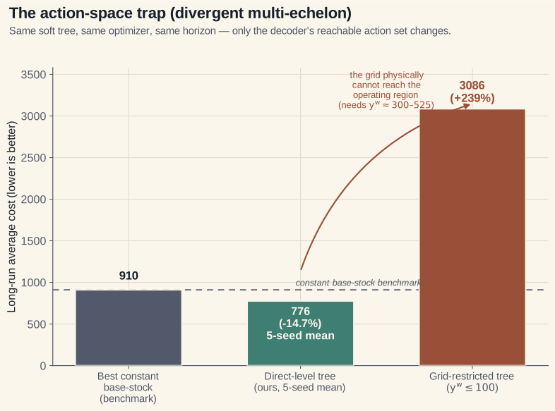
One honesty caveat I keep explicit: the 14.7% / 12.0% figures are measured against the best in-environment constant base-stock under one cost convention, whereas the published A3C improvements (8.95%, 12.09%) are against a different baseline under a different cost convention. So the A3C comparison is cross-protocol context — indicative of the direct design’s strength, not a strictly like-for-like ranking or a head-to-head beat.
Perishable inventory — beats the best base-stock gate
Stock ages and expires; a waste cost is charged on outdated units. The benchmark instances issue either FIFO or LIFO. A 21-parameter age-dependent soft tree beats the best base-stock gate under a shared common-random-number estimator, and the beat is seed-robust: over five independent CMA-ES seeds the improvement is +1.171% ± 0.002% under FIFO and +0.840% ± 0.034% under LIFO, with all five seeds beating the gate on both — the cross-seed std is negligible against the mean margin. The tree exploits the age structure a single base-stock cannot — ordering less when older stock is already on hand. (Both learned returns happen to sit essentially on the analytic value-iteration optimum, but that comparison mixes two estimators, so I treat it as corroborating context, not a second win.)
General-network backorder — beats the published benchmark by over 20%
A four-warehouse, five-retailer network (the Geevers et al. (2024) CardBoard instance) with backordered (not lost) demand. Put the policy in the node-base-stock-targets coordinate system and let a state-dependent tree modulate the targets, and it reduces long-run average cost by 24.3% ± 1.8% over the reproduced constant node-base-stock benchmark (gate 10,354.8; learned five-seed mean 7,837.0 ± 189.7, all five seeds below by 23–27%), on the same environment under a paired comparison. The same recipe on the Kunnumkal–Topaloglu divergent instance gives an even larger, tighter beat: 36.8% ± 0.3% over its reproduced gate (3,930.4), again with all five seeds below. These are seed-robust means, not best-of-N.
Two honest caveats. First, despite the family name, this verified environment charges holding and backorder cost only — no fixed ordering cost. Second, the paper’s PPO best (8,714) is a cross-protocol figure produced by a different learner under its own protocol. All five of our seeds land below it, but that is not a head-to-head PPO beat and I do not claim one — the defensible claim is the paired, same-environment improvement over the published constant base-stock benchmark.
Serial multi-echelon (Clark–Scarf) — matches the proven optimum
A 3-stage serial system whose optimal policy is known exactly (Clark–Scarf echelon base-stock). Because the decoder lives in the optimum’s own coordinate system, the warm-started direct-level soft tree reproduces the proven optimum to within +0.011% — inside the environment’s own ~0.06% reproduction band, statistically indistinguishable from optimal. This is a match, not a win: one cannot improve on a true optimum, and I do not claim to. What it shows is that the same generic recipe recovers the optimal policy on a serial system.
One-warehouse multi-retailer — beats the tuned gate, but below published PPO
Asymmetric, high-variability OWMR instances from Kaynov et al. (2024). The like-for-like comparator is a strong in-repo tuned base-stock-plus-allocation gate (itself already stronger than the published Kaynov base-stock). Under the seed-robust standard the learned per-retailer soft tree now robustly beats the tuned gate on all three asymmetric / high-variability rows, with every seed below the gate: the asymmetric three-retailer instance by +4.61% (five-seed mean 1115.67 ± 6.13 vs gate 1169.59), the high-CV ten-retailer instance by +7.07% (five-seed mean 85,395 ± 1031 vs 91,890.25), and the previously-unsolved strongly heterogeneous ten-retailer instance by +12.44% (five-seed mean 44,170.26 ± 450.4 vs 50,445.20). That hardest instance is exactly the one the hand search could only tie until the automated structure search cracked it — once the geometry is searched rather than hand-picked (below). On three further $K{=}3$ backorder / lost-sales regime rows the same tree matches (ties) the tuned gate rather than beating it — reported honestly as gate-matches.
To be clear about the ceiling: the learned policy does not robustly beat the published PPO, which remains the strongest learned reference (on the high-CV row the seed-mean is ~7% above PPO; on the hardest heterogeneous row the 44,170.26 seed-mean sits ~3% above the published PPO scalar 42,835.02). PPO is cross-protocol context only; the win is over the tuned heuristic gate, not over published deep RL.
Ameliorating inventory — beats the order-up-to gate; the LP value is an upper bound
Here stock improves with age (think spirits, port wine) and the objective is long-run average profit with a stochastic purchase price. A price-reactive linear-leaf soft tree — buy more when the realized price is low, which a fixed order-up-to level cannot do — beats the best tuned order-up-to gate by a wide margin (+450% and +278% of the gate’s profit, with overwhelming statistical significance).
The other reference point is a perfect-information LP upper bound, and I treat it as exactly that. The remaining gap to it is large (94.2% and 79.3%) and structural: the bound assumes hindsight and a full three-part decision (purchase, production, per-age issuance solved jointly), while our policy controls only the scalar purchase volume. So the bound is reported as a gap, never “beaten”, and it is not comparable to the ~3.5% gap a full-action-space deep-RL agent reaches.
Production / assembly / distribution network — a research result on a faithful environment
A 3-node serial production chain (plus two further topologies below). The honesty status matters: this environment faithfully reproduces the one published single-node quantity (certifying its dynamics), but there is no published optimum for the multi-node MDP — and no published DRL/PPO baseline at all — so the comparator is the environment’s own best heuristic (a grid-searched pairwise base-stock), not a literature number. Against that gate on the serial chain, the learned linear-leaf soft tree improves per-period cost by −4.96% / −8.77% (two seeds, depth 2) and −3.97% (depth 3), every configuration robustly outside the held-out standard error (≥ 10× SEM).
The same recipe carries to two harder topologies of the same supply-network model: on a pure assembly network the tree beats the gate by −2.98% (274.90 vs 283.34, ≈40× SEM); and on the mixed distribution-plus-assembly network, the new residual gate-backbone head (below) turns a gate-match into a robust −2.20% gate-beat (five-seed mean 291.14 ± 2.49 vs 297.69, all five below).
I frame this honestly as a research result on a faithful-but-not-literature-anchored environment — the policy beats the environment’s own best heuristic on the serial, pure-assembly, and mixed topologies, not any published cost or DRL number. It is evidence for the same thesis as everywhere else: action design (here, the leaf class and the decoder head) governs whether a black-box search recovers structured-control performance.
What ties it together
The same gradient-free loop, run with one fixed configuration and no per-problem tuning, produces the picture below. The improvements span wildly different scales and three different kinds of comparator, so a single bar chart of ”% improvement” would be misleading. Instead each problem is read by its honest verdict — match a proven optimum, beat a heuristic, report a gap to an upper bound, or a research result on a faithful environment:
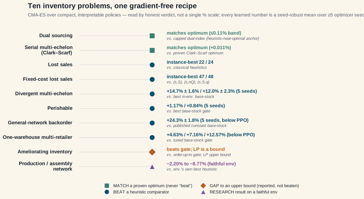
The same data, with the comparator made fully explicit:
| Problem | Comparator | Honest verdict |
|---|---|---|
| Lost sales | classical heuristics | instance-best in 22/24 |
| Fixed-cost lost sales | $(s,S)$, $(s,nQ)$, $(s,S,q)$ | instance-best in 47/48 |
| Dual sourcing | capped dual-index (heuristic-near-optimal anchor) | matches the proven optimum (seed-robust; +0.09%…+0.96% vs CDI, no robust beat) |
| Divergent multi-echelon | best in-env. base-stock | beats by 14.7% ± 1.6% / 12.0% ± 2.3% (5 seeds, all below; A3C indicative context) |
| Perishable | best base-stock gate | beats the gate (+1.171% ± 0.002% / +0.840% ± 0.034%, 5 seeds) |
| General-network backorder | published constant base-stock | beats by 24.3% ± 1.8% (set 1) / 36.8% ± 0.3% (KT), 5 seeds (below PPO, not a PPO beat) |
| Serial (Clark–Scarf) | proven optimum | matches the proven optimum (+0.011%) |
| One-warehouse multi-retailer | tuned base-stock gate | beats the gate on all three rows: +4.61% / +7.07% / +12.44% (the hard instance_14 via structure search; ~3% above PPO, not a PPO beat) |
| Ameliorating | order-up-to gate; LP bound | beats the gate (+450% / +278%); LP value is an upper bound |
| Production network | env.’s own best heuristic | beats it (serial −4.96%…−8.77%; pure-assembly −2.98%; mixed net robust −2.20% via the residual gate-backbone head; no published DRL — gate-beat only) |
The policies that produce this carry tens to a few hundred parameters — orders of magnitude fewer than published DRL networks — and the reported single-state actions are validated against an independent rollout, so they are not just compact but checkable.
Two limitations are worth stating plainly. The high-penalty, autocorrelated MMPP lost-sales instances at the longest lead times stay won by classical heuristics — a real gap for stationary compact policies under regime-switching demand. And CMA-ES, while far more sample-efficient than A3C here, is still data-hungry relative to limited-data settings, and its population evaluation cost grows with the covariance dimension, so very large parameterizations would need restricted or separable covariance structures.
Searching for the action geometry — and a new one that cracks the last network
Everything above shares a quiet assumption: I hand-designed each decoder, reading the relevant heuristic and shaping the action geometry to match. If the action parameterization really is the policy, then the natural next move is to make the choice of geometry itself something you search — and to do it under the same honest gate. Two results came out of taking that seriously.
Automating the structure search. I built an agentic loop in which an LLM agent (Codex, driven through a small framework) proposes policy structures — the action head, the per-dimension geometry, the split type, the leaf class, the feature basis — as short specs in a tiny DSL. Each proposed spec is compiled to an invman soft-tree policy, warm-started at a gate-invertible anchor (so generation zero reproduces the heuristic gate exactly), tuned by the same inner CMA-ES on the same Rust rollout oracle, and then scored seed-robustly against the gate. The outer loop is an evolutionary archive: keep a spec only if it is a robust gate-beat — every one of five optimizer seeds below the gate and mean-plus-std below the gate. The agent proposes the structure; CMA-ES still owns the continuous parameters; the keep decision stays deterministic and honest. The one wrinkle worth noting is that a naive proposer fixates: once a structure is the archived best, it keeps re-proposing it. Adding novelty pressure — diverse elites (the best spec per structural niche) plus an anti-repeat rule that forces each proposal to differ from the incumbent on at least one structural axis — broke that plateau, and broke it productively.
A hard instance, now robustly beaten. The spearhead was the one-warehouse multi-retailer instance the hand search could only tie (instance_14, the asymmetric high-variability case above). The fixated short run settled on a linear-leaf structure that beat the gate by a modest margin. The novelty-driven longer run surfaced a structure the short run never tried — a constant leaf, oblique split, per-retailer echelon_targets head — that the agent reached by mutating off its own incumbent. At full budget over five optimizer seeds it lands at a seed-robust mean of 44170.26 versus the in-repo echelon-base-stock gate of 50445.20 — a −12.44% gate-beat, with 5/5 seeds below the gate and a std of 450.4 (about 1.0% of the mean). The same honesty caveat as before still binds, and it matters here: the published PPO scalar (Kaynov et al., 2024; ≈42835) is cross-protocol context only, and we sit about 3% above it. This is a robust beat over the tuned heuristic gate on a previously-unsolved instance — not a PPO beat, and I do not claim one.
A new action geometry — the residual gate-backbone head. The production network’s mixed distribution-plus-assembly variant was the lab’s genuinely open case: hand-search with the older vector_quantity head only ever tied its gate (seed-mean 306.10 ± 22.89, +2.8%, 4 of 8 seeds below — parity, not a beat). The diagnosis was structural: that head’s scale-normalized leaf is not gate-invertible, so there is no clean gate-reproducing warm-start and the optimizer seeds scatter by ±22.9. The fix is a new decoder, the residual gate-backbone head: the order is $\text{clamp}(\text{gate_order} + \text{round}(\delta),,0,,\text{max})$ with the learned residual $\delta = 0$ at zero parameters — so generation zero reproduces the gate byte-exact (proven by an in-crate test) and every optimizer seed is anchored at the gate by construction. With this head (linear leaf, oblique split, per-relation, warm-started at $\delta=0$), the agentic search produces a seed-robust mean of 291.136 versus the env’s own pairwise base-stock gate of 297.688 — a −2.20% gate-beat, with 5/5 seeds below the gate (287.36, 294.42, 290.74, 293.22, 289.93) and a std of 2.49. The headline is not just the margin but the variance: anchoring every seed at the gate collapsed the seed scatter from ±22.9 to 2.49, turning a network that hand-search could only tie into a robust beat. The production network has no published DRL or PPO baseline at all, so this is a gate-beat only — a research result against the environment’s own best heuristic, never any DRL claim.
The point of this turn is the same as the one the next section describes the field taking. When the structure search itself becomes part of the system — and especially when the search invents a decoder, like the residual gate-backbone, that anchors the optimizer at the heuristic and learns only the deviation — the structure has gone all the way back into the policy. The action parameterization is still the policy; we have just stopped hand-picking it.
Where this fits, and where the field is going
It helps to place this work on the map of how inventory control has been learned over the last few years, because the throughline of that map is exactly the lever this post leans on.
Two starting points. Classical inventory theory gives us structured heuristics — base-stock, $(s,S)$, dual-index, capped dual-index — each derived from a structural property of the optimal policy, each strong but narrow. The deep-RL line, opened up for inventory by the roadmap of Boute et al. (2022) and the cross-problem A3C study of Gijsbrechts et al. (2022), went the other way: hand a large neural network the raw problem and let it discover structure from simulated experience. That generality is real, and later work pushed it onto harder systems — PPO for one-warehouse multi-retailer (Kaynov et al., 2024) and multi-echelon (Geevers et al., 2024). But it came at a price the roadmap itself names: heavy tuning, large and opaque networks, and results that are hard to reproduce and compare across papers.
The turn the field is taking: structure goes back into the policy. The most striking thing in the recent literature is that the strongest learners have stopped trying to free a big network to discover structure and have started injecting structure into the learner. Maggiar et al. (2025) build structure-informed policy networks that bake monotonicity and other analytically known properties of optimal policies directly into the architecture. Temizoz et al. (2025) report that their model-based deep controlled learning scheme reaches optimality gaps of at most 0.2% on lost-sales and perishable problems — far inside the gaps earlier A3C reached — using a single fixed hyperparameter set. And a growing set of agents simply make the parameters of a classical control the action space itself. These are independent groups, with different machinery, all converging on the same idea: structure in the policy beats capacity in the network.
That is precisely the lever in this post, reached from the gradient-free side. The “action parameterization is the policy” idea — putting the search directly in the heuristic’s coordinate system and letting a tiny model modulate it — is the same principle expressed as a design choice rather than a regularizer baked into a network. The multi-echelon action-space trap is the cleanest evidence I have for why it matters: hold the learner fixed and only the coordinate system the decoder lives in decides whether you land 14% better than the best base-stock or 200% worse. Seen this way, evolution strategies are not a competitor to the structure-informed DRL line so much as a different point on the cost–complexity frontier that reaches the same conclusion — and the black-box-search tradition it comes from (Salimans et al., 2017; Mania et al.’s 2018 finding that even linear policies from simple random search are competitive on hard control benchmarks) suggests the conclusion is robust to how you do the optimizing.
The field’s second worry: reproducibility and comparability. A recurring complaint in this literature is that DRL inventory “wins” are hard to trust because cost conventions, demand processes, and baselines differ from paper to paper, and there is no ImageNet-style standard benchmark (Boute et al., 2022; Alvo et al., 2023). Alvo et al.’s HDPO work makes the constructive point that inventory is actually unusually well-suited to reliable evaluation, because in several problem classes you can compare a learned policy to the optimum itself, not merely to another learner. The discipline in this post is a small contribution in that spirit: every environment is anchored to a published number before it carries any learned claim, and every result is reported under one of three honest verdicts — match a proven optimum (dual sourcing, serial Clark–Scarf; never “beat”), beat a heuristic (where the margin clears the held-out standard error under common random numbers), or report a gap to an upper bound without ever calling it beaten (ameliorating inventory’s perfect-information LP). Where the comparator is published deep RL we sit below it (one-warehouse multi-retailer, the general-backorder cross-protocol figure) and say so. The aim is not to top a leaderboard but to state exactly what kind of claim each number supports.
There is also a theory reason to prefer small. Xie et al. (2024) bring VC theory to inventory policies and show that structured classes generalize from limited data: the generalization error of a base-stock class is essentially independent of the horizon, and only logarithmic for $(s,S)$ — “learning less is more.” A policy with a few hundred parameters living in a heuristic’s coordinate system is squarely the kind of low-complexity class those guarantees cover, which is reassuring when your training signal is a finite simulation rather than an asymptotic average.
Where it’s heading, and the open directions. Three currents seem to me to define the near future, and they suggest the natural next steps for this line of work:
- Reproducible, optimum-anchored benchmarks. The field wants open environments compared to known or bounded optima rather than to other learners (Alvo et al., 2023; Temizoz et al., 2025). Contributing a suite of literature-validated environments with the three-verdict accounting baked in is the obvious next move.
- Interpretable, compact policies as a first-class goal. Auditability and deployability are now stated objectives, not afterthoughts — and the VC-theory result says compactness is a statistical asset, not just an engineering convenience.
- Hybridizing action geometry with sample-efficient learners. The cleanest synthesis is to hand a gradient-based learner the same policy-owned decoders, using a heuristic warm-start (as done here for dual sourcing, serial multi-echelon, and general-network backorder) or CMA-ES to seed, and a sample-efficient learner to refine. That directly targets the two places this recipe still loses: the long-lead autocorrelated MMPP lost-sales instances, and the below-PPO gap on one-warehouse multi-retailer.
- Generalist and limited-data settings. The frontier is turning toward generally-capable agents trained for zero-shot transfer across instances and then paired with estimate-then-decide adaptation at deployment (Temizoz et al., 2024). The favorable sample complexity of structured policy classes suggests these compact decoders are exactly the right hypothesis class for the data-scarce regime — amortize one decoder across an instance family rather than retraining per instance.
The through-line, in one sentence: in inventory control the representation of the action is at least as consequential as the choice of learner — and a compact, honest, reproducible policy is often enough.
Takeaways
- A single, generic recipe — CMA-ES over small, interpretable policies — is competitive across ten classical inventory problems, with little tuning.
- The consequential design choice is the decoder and its action geometry, not the network size: shape the decoder like the relevant heuristic’s coordinate system and a tiny policy reaches the good operating region.
- Read the verdicts honestly: match where the comparator is a proven optimum (dual sourcing, serial Clark–Scarf), beat where the comparator is a heuristic, and below published deep RL where one exists. Understatement is the right default.
Citation
If you find this work useful, please cite it as:
@article{ManafInventoryES,
  title   = "Learning Inventory Control Policies with Evolution Strategies across Lost-Sales, Dual-Sourcing, and Multi-Echelon Problems",
  author  = "Manaf, Nima",
  journal = "nimamanaf.com",
  year    = "2026",
  url     = "https://nimamanaf.com/posts/learning-to-control-inventory-management-systems"
}